
TL;DR
- What It Is: The operational phase of machine learning, known as AI inference, consists of using a trained model to generate outputs like text, images, or predictions from new data.
- Inference vs. Training: Training is the process of building the model with a lot of upfront compute. Inference is the ongoing execution of that model. Inference often consumes the lion’s share of long-term AI budgets because it runs continuously for every user request.
- How LLM Inference Works: Large Language Model (LLM) inference consists of two phases: the Prefill Phase (processing the prompt, driving Time to First Token) and the Decode Phase (generating response tokens one by one).
- Types of Workloads: Inference is categorized by latency and throughput needs, including Real-Time (chatbots, voice agents), Batch (large document processing), Streaming, and Edge (on-device) inference.
- Performance & Cost Drivers: Enterprise AI costs are impacted by model size, context length, GPU utilisation, and the latency-throughput tradeoff (speed per request versus overall volume processed).
- Optimization Techniques: Engineering teams reduce inference costs and speed up inference with techniques such as quantization (FP8/INT4), continuous batching, KV caching, and smart autoscaling.
Inference in AI is the process of taking a trained model and running it on new input to produce an output, a prediction, a classification, some generated text, or an image. Training is when the model learns; inference is when the model is actually doing the work, every time a user or system sends a request. With Deloitte predicting that inference will account for roughly two-thirds of all AI compute in 2026, understanding this phase matters for engineering and product teams. In this guide, we’ll cover how AI inference works, key metrics for performance, and real-world strategies for production optimisation.
What Happens When You Ask ChatGPT a Question?
Yes, every ChatGPT reply is inference. Here's roughly what happens when you hit enter:
- Your message is split into tokens and sent to a GPU server running the model.
- The model reads the whole prompt in one pass and stores intermediate results in memory (the KV cache).
- It predicts the first token of the reply. That moment is what engineers call time to first token.
- It then generates the rest of the reply one token at a time, reusing the cached results so it doesn't re-read your whole prompt for every word.
- Each token is streamed back to your screen as it's produced.
None of this changes the model. Ask the same question tomorrow and the same weights answer it. Any "learning" from your conversation happens later, if at all, through a separate training or fine-tuning process.
AI inference vs. the everyday meaning of "inference": In everyday English, an inference is a conclusion you reach from evidence ("she's wearing a coat, so it's probably cold"). AI inference borrows the idea, but here it refers to the computational process of running a model. When engineers talk about "inference cost" or "inference latency," they mean compute and time, not reasoning skill.
Understanding AI Inference: Definition and Examples
Inference is the process where you take a trained machine learning model, and then you use that model to generate outputs or predictions on new data or unseen data. For example, an email spam filter that looks at an incoming message and determines it is spam, or a smartphone photo app that can recognise a face in a new image, is doing inference.
To see for different modalities:
- Text/LLMs: An AI model answers an incoming prompt, generating one token at a time.
- Audio: A spoken lecture is transcribed to text by a speech-to-text model such as Whisper.
- Vision/Diffusion: A generative model is given a text prompt, and it generates a brand new image.
- Classify: A traditional ML model assigns a score to an incoming email to decide if it is spam.
What is Inference in Generative AI?
Generative AI describes what a model does: it creates new text, images, audio, or code. Inference describes when it does it. Every output from a generative model is produced during inference. Training built the model; inference is the model at work.
Key Takeaway: Training builds the model with heavy upfront compute; inference is the model at work executing on live inputs.
Machine Learning Inference vs. Statistical Inference
In classical statistics, inference involves concluding about a population from a sample dataset. In machine learning, however, inference refers strictly to executing a trained computational graph on live inputs to generate predictions or content.
AI Inference vs. Training: Key Differences Explained
What Is the Difference Between ML Inference and LLM Inference?
Both are inferences, but they behave like different workloads. Classic ML inference (a fraud classifier, a recommendation model, an image tagger) runs one forward pass and returns a fixed-size answer. LLM inference generates its answer one token at a time, so a single request can mean hundreds or thousands of forward passes.
Why Are LLMs Harder to Serve Than Traditional ML Models?
Three things make LLM serving harder than serving classic ML models:
- Request cost is unpredictable. Two prompts of the same length can produce answers 20 tokens or 2,000 tokens long. Capacity planning has to account for output length, not just request count.
- Memory is the real constraint. Model weights take up much of the GPU memory, and each active request also holds a KV cache. How many users a GPU can serve at once is often limited by memory, not compute.
- The two phases pull in opposite directions. Reading the prompt is compute-heavy, while generating tokens is memory-bound. NVIDIA's Dynamo documentation makes exactly this distinction when explaining why some teams now run the two phases on separate GPU pools.
When Does a Traditional ML Model Still Make More Sense?
Not every problem needs an LLM. If the output is a score, a category, a forecast or an embedding, a smaller specialized model is usually faster and far cheaper to run.
Lyric, a supply-chain planning platform, is a good example. It serves time-series forecasting models (Chronos, TimesFM) and an embedding model (Stella) rather than a chat LLM. Its challenges were large tensor payloads and slow scale-up from zero. After moving to Simplismart, its embedding latency dropped from about 500ms to about 40ms and cold starts fell from about 300 seconds to about 75 seconds. Inference engineering applies to these models just as much as to LLMs.
How Does AI Inference Work? The 7-Step Production Lifecycle
Every inference request, from the moment a user hits send to the final streamed token, traverses a rigorous, multi-stage path through the network, serving edge, and GPU execution engine.
Step 01: User Query & Wire Format Transport
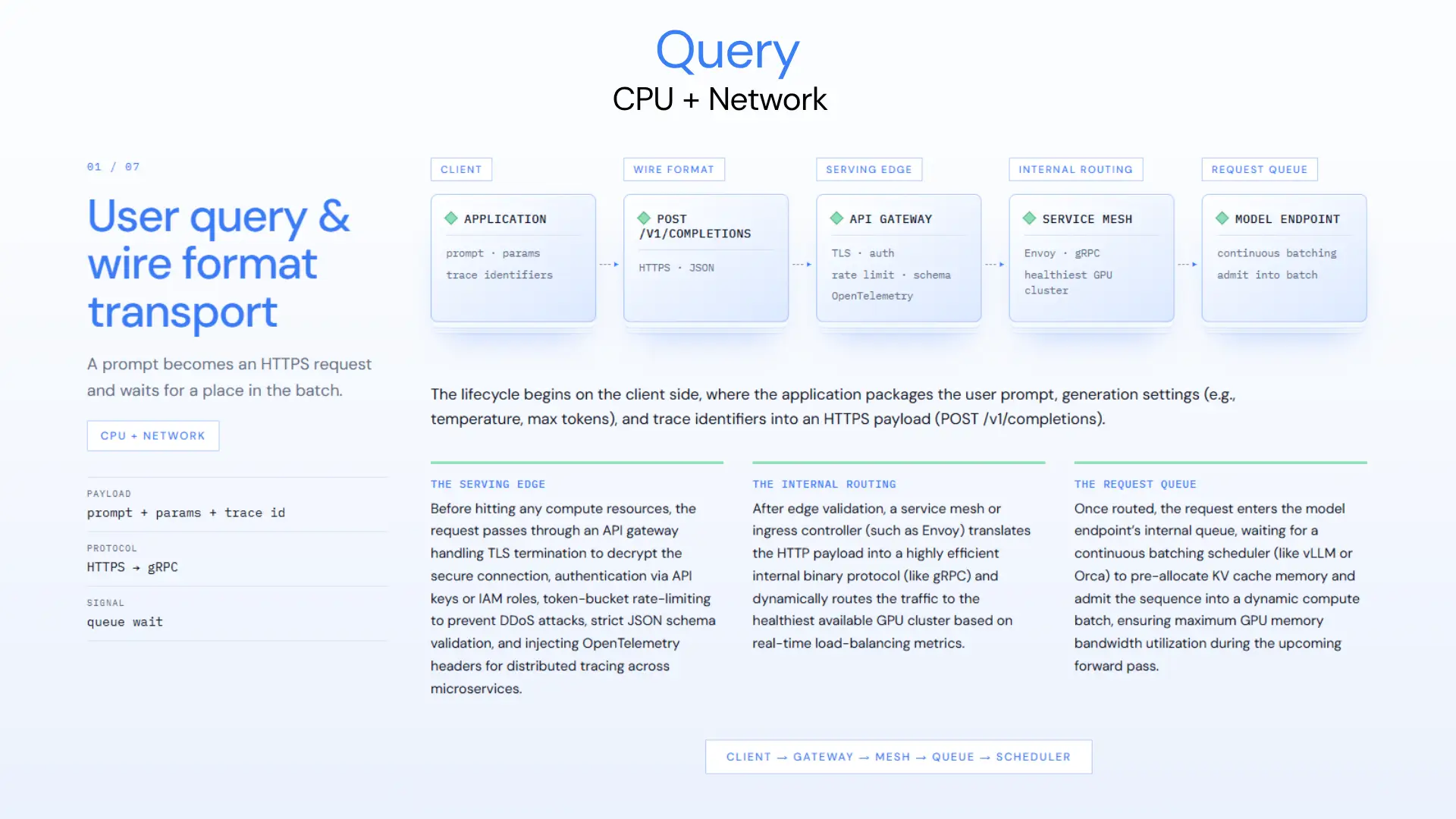
The lifecycle begins on the client side, where the application packages the user prompt, generation settings (e.g., temperature, max tokens), and trace identifiers into an HTTPS payload (POST /v1/completions).
- The Serving Edge: Before hitting any compute resources, the request passes through an API gateway handling TLS termination to decrypt the secure connection, authentication via API keys or IAM roles, token-bucket rate-limiting to prevent DDoS attacks, strict JSON schema validation, and injecting OpenTelemetry headers for distributed tracing across microservices.
- The Internal Routing: After edge validation, a service mesh or ingress controller (such as Envoy) translates the HTTP payload into a highly efficient internal binary protocol (like gRPC) and dynamically routes the traffic to the healthiest available GPU cluster based on real-time load-balancing metrics.
- The Request Queue: Once routed, the request enters the model endpoint’s internal queue, waiting for a continuous batching scheduler (like vLLM or Orca) to pre-allocate KV cache memory and admit the sequence into a dynamic compute batch, ensuring maximum GPU memory bandwidth utilization during the upcoming forward pass.
Step 02: Tokenization & Vocabulary Lookup
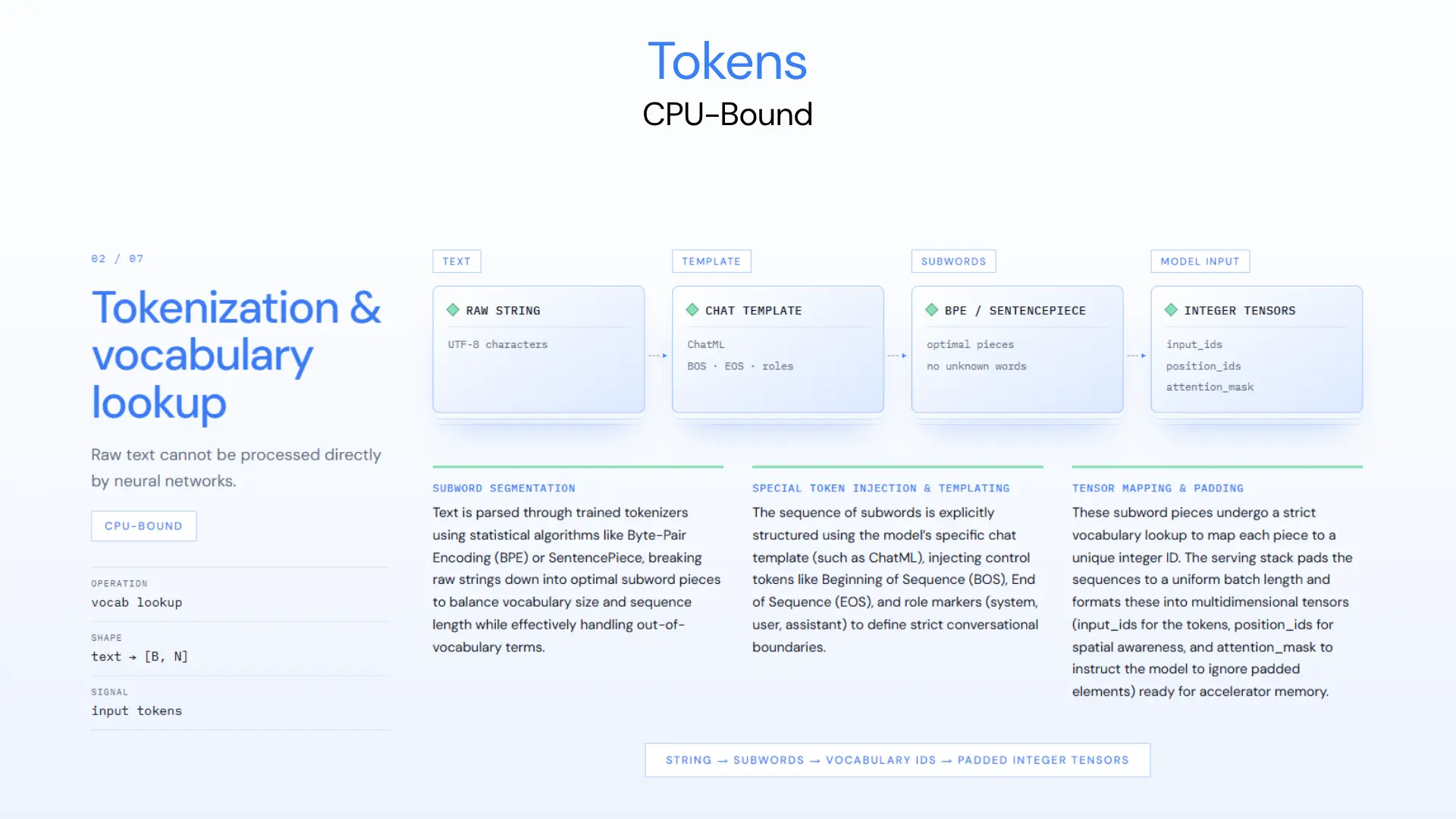
Raw text cannot be processed directly by neural networks.
- Subword Segmentation: Text is parsed through trained tokenizers using statistical algorithms like Byte-Pair Encoding (BPE) or SentencePiece, breaking raw strings down into optimal subword pieces to balance vocabulary size and sequence length while effectively handling out-of-vocabulary terms.
- Special Token Injection & Templating: The sequence of subwords is explicitly structured using the model's specific chat template (such as ChatML), injecting control tokens like Beginning of Sequence (BOS), End of Sequence (EOS), and role markers (system, user, assistant) to define strict conversational boundaries.
- Tensor Mapping & Padding: These subword pieces undergo a strict vocabulary lookup to map each piece to a unique integer ID. The serving stack pads the sequences to a uniform batch length and formats these into multidimensional tensors (input_ids for the tokens, position_ids for spatial awareness, and attention_mask to instruct the model to ignore padded elements) ready for accelerator memory.
Step 03: The Prefill Phase (Compute-Bound)
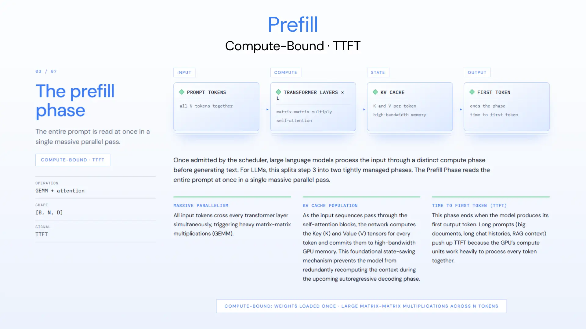
Once admitted by the scheduler, large language models process the input through a distinct compute phase before generating text. For LLMs, this splits step 3 into two tightly managed phases. The Prefill Phase reads the entire prompt at once in a single massive parallel pass.
- Massive Parallelism: All input tokens cross every transformer layer simultaneously, triggering heavy matrix-matrix multiplications (GEMM).
- KV Cache Population: As the input sequences pass through the self-attention blocks, the network computes the Key (K) and Value (V) tensors for every token and commits them to high-bandwidth GPU memory. This foundational state-saving mechanism prevents the model from redundantly recomputing the context during the upcoming autoregressive decoding phase.
- Time to First Token (TTFT): This phase ends when the model produces its first output token. Long prompts (big documents, long chat histories, RAG context) push up TTFT because the GPU's compute units work heavily to process every token together.
Step 04: KV Cache & Memory Management
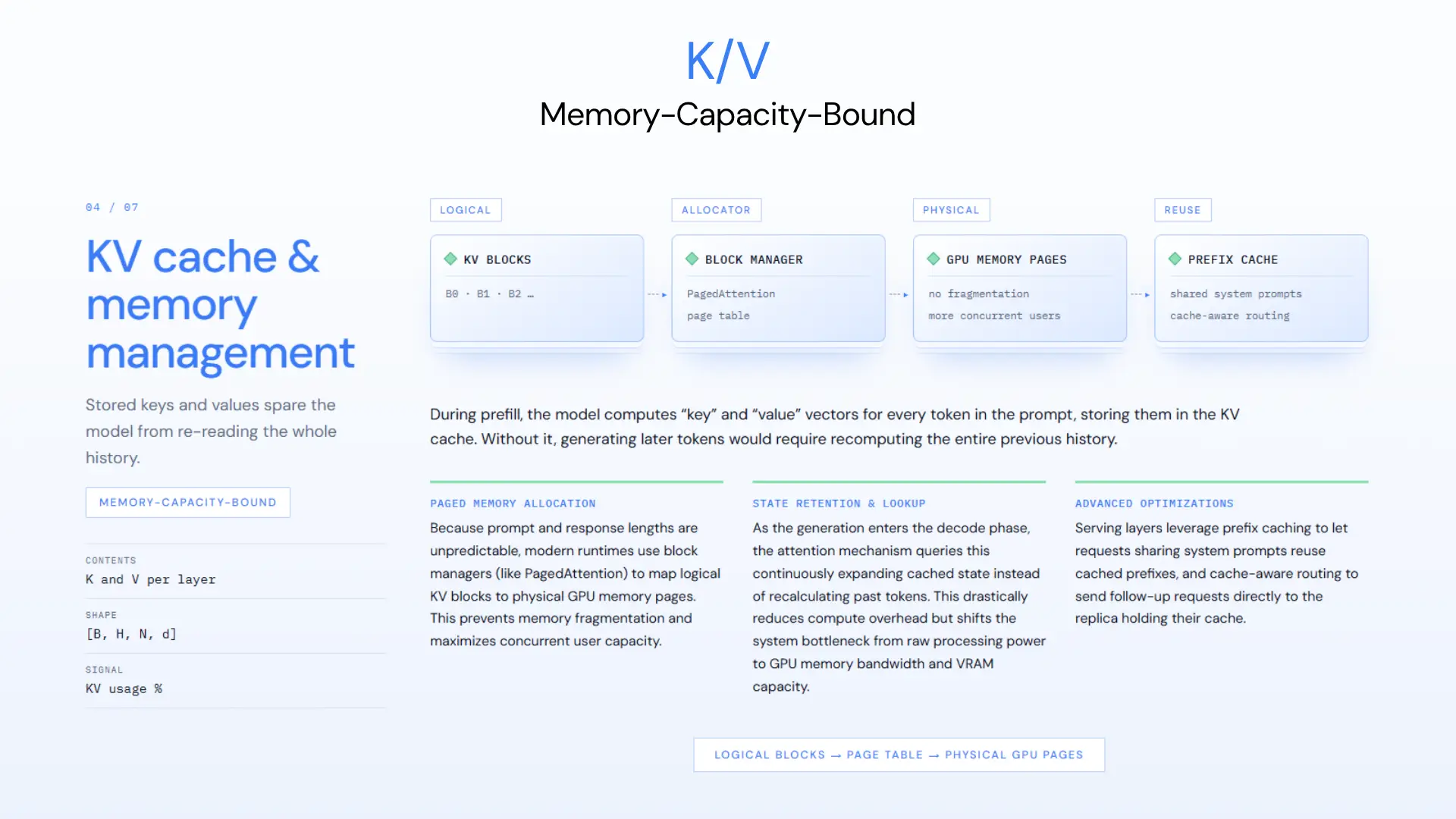
During prefill, the model computes "key" and "value" vectors for every token in the prompt, storing them in the KV cache. Without it, generating later tokens would require recomputing the entire previous history.
- Paged Memory Allocation: Because prompt and response lengths are unpredictable, modern runtimes use block managers (like PagedAttention) to map logical KV blocks to physical GPU memory pages. This prevents memory fragmentation and maximizes concurrent user capacity.
- State Retention & Lookup: As the generation enters the decode phase, the attention mechanism queries this continuously expanding cached state instead of recalculating past tokens. This drastically reduces compute overhead but shifts the system bottleneck from raw processing power to GPU memory bandwidth and VRAM capacity.
- Advanced Optimizations: Serving layers leverage prefix caching to let requests sharing system prompts reuse cached prefixes, and cache-aware routing to send follow-up requests directly to the replica holding their cache.
Step 05: The Decode Phase (Memory-Bandwidth Bound)
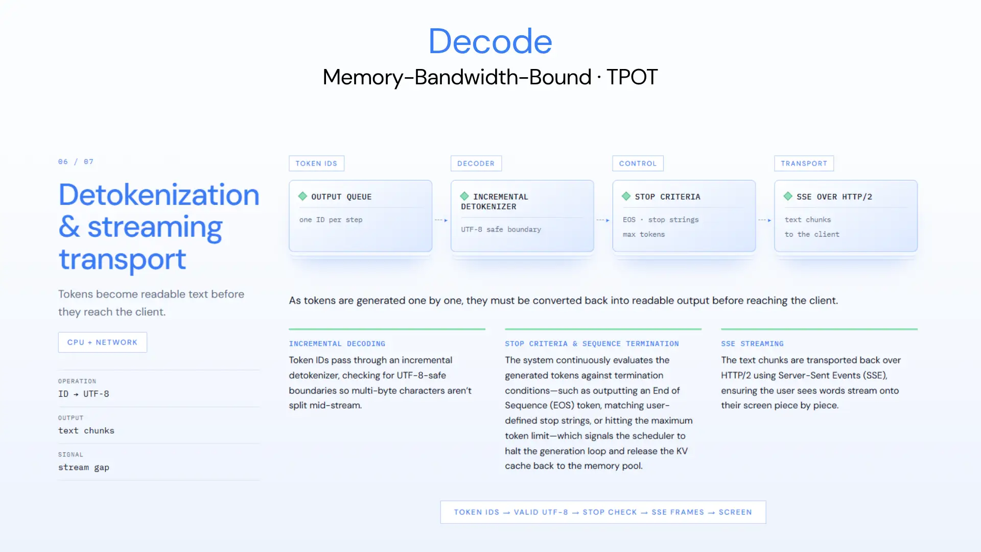
Following prefill, the model enters the Decode Phase, generating the answer one token at a time.
- Sequential Iteration: Each new token requires another pass through the model for that single token. Very little compute happens per step, but the full model weights and KV cache must be read from memory every time.
- Logits Processing & Sampling: At the end of each forward pass, the model outputs a probability distribution (logits) across the entire vocabulary. The serving layer applies the user's specific generation parameters (such as temperature, top-k, and top-p) to sample the final token, which is then appended to the active sequence and KV cache for the next iteration.
- Bottlenecks & Metrics: Decode is strictly limited by memory bandwidth, and its speed is measured in Tokens per Second / TPOT (Time Per Output Token). Because long prefills can stall other users' decode steps on the same GPU, modern stacks handle this with chunked prefill, disaggregated GPU pools, or frameworks like vLLM and TensorRT-LLM.
Step 06: Detokenization & Streaming Transport
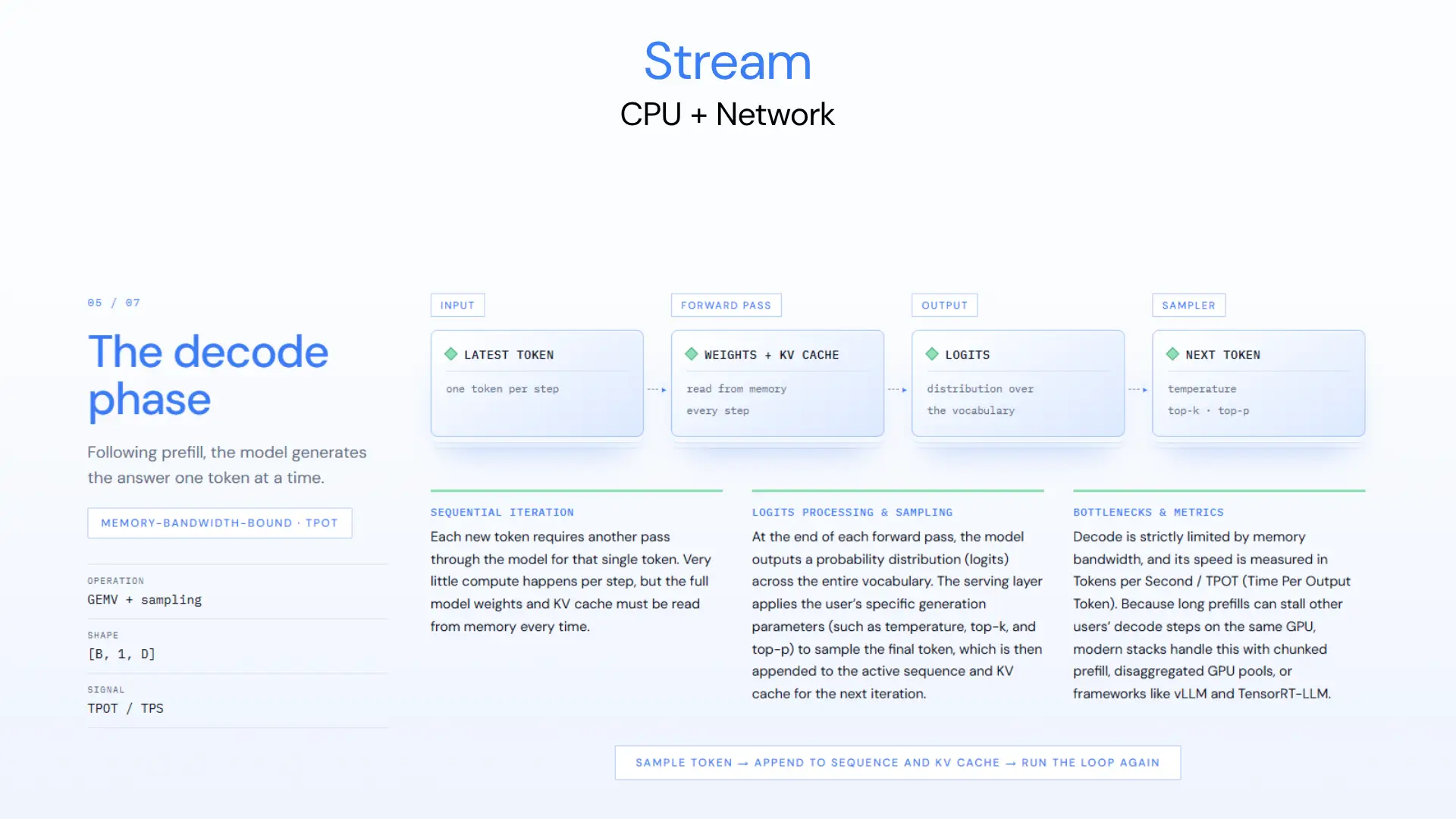
As tokens are generated one by one, they must be converted back into readable output before reaching the client.
- Incremental Decoding: Token IDs pass through an incremental detokenizer, checking for UTF-8-safe boundaries so multi-byte characters aren't split mid-stream.
- Stop Criteria & Sequence Termination: The system continuously evaluates the generated tokens against termination conditions—such as outputting an End of Sequence (EOS) token, matching user-defined stop strings, or hitting the maximum token limit—which signals the scheduler to halt the generation loop and release the KV cache back to the memory pool.
- SSE Streaming: The text chunks are transported back over HTTP/2 using Server-Sent Events (SSE), ensuring the user sees words stream onto their screen piece by piece.
Step 07: Production Inference Serving & Orchestration
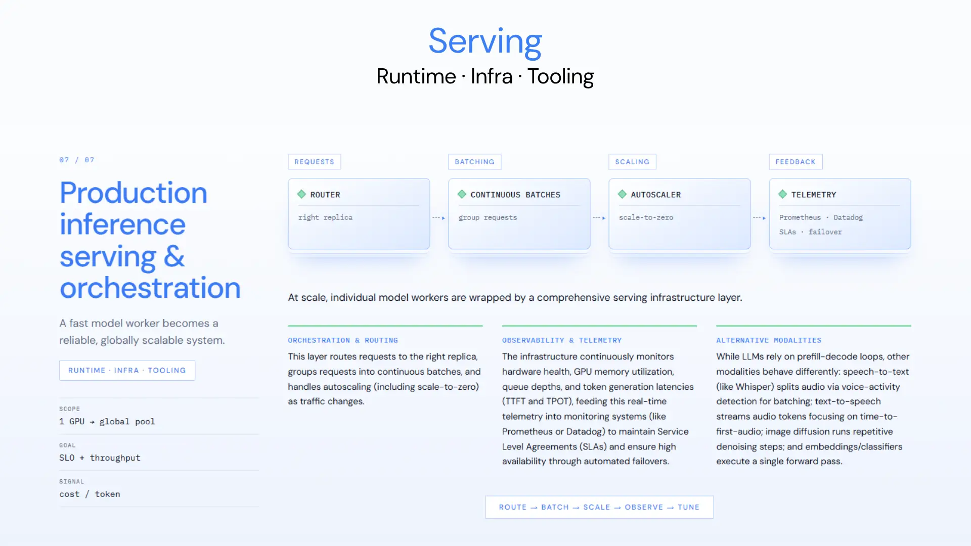
At scale, individual model workers are wrapped by a comprehensive serving infrastructure layer.
- Orchestration & Routing: This layer routes requests to the right replica, groups requests into continuous batches, and handles autoscaling (including scale-to-zero) as traffic changes.
- Observability & Telemetry: The infrastructure continuously monitors hardware health, GPU memory utilization, queue depths, and token generation latencies (TTFT and TPOT), feeding this real-time telemetry into monitoring systems (like Prometheus or Datadog) to maintain Service Level Agreements (SLAs) and ensure high availability through automated failovers.
- Alternative Modalities: While LLMs rely on prefill-decode loops, other modalities behave differently: speech-to-text (like Whisper) splits audio via voice-activity detection for batching; text-to-speech streams audio tokens focusing on time-to-first-audio; image diffusion runs repetitive denoising steps; and embeddings/classifiers execute a single forward pass.
4 Types of AI Inference Workloads
Inference type comparison
Different workloads require different execution paradigms depending on latency and throughput constraints:
Real-time (Online) Inference
Real-time inference is optimized for instantaneous responses where sub-second latency is critical. This setup requires high baseline compute capacity to handle immediate user requests, making it the standard for conversational chatbots, real-time voice agents, and it also includes live fraud detection systems.
Batch (Offline) Inference
Batch inference is the process of running inference on large amounts of data at once, typically during off-peak hours to maximise throughput and hardware efficiency. This method is well suited for non-real-time applications such as scoring documents nightly, large translation pipelines, and large queues of transcriptions.
Streaming and Asynchronous Inference
Streaming inference is meant for ongoing data pipelines, where data chunks are fed as soon as they are available. This paradigm is a good match for real-time Text-to-Speech (TTS) and Speech-to-Text (STT) applications as well as long-running asynchronous analysis jobs that scale with active streams.
Edge and On-Device Inference
Edge inference runs AI models on local hardware, so it doesn't require constant cloud connectivity. It is purpose-built for environments with hard power, compute, and latency constraints and is the go-to solution for mobile phones, smart cameras, and industrial factory sensors.
AI Inference Deployment Options: Cloud, On-Prem, and Edge
Teams deploy inference across various infrastructure topologies depending on security, cost, and control requirements:
- Shared model APIs: Pay-per-token pricing managed entirely by third-party providers.
- Dedicated deployments: Single-tenant cloud instances billed per GPU hour.
- Bring Your Own Cloud (BYOC): Running managed infrastructure inside your own secure AWS, GCP, or Azure cloud account.
- On-premises: Infrastructure that sits inside the company's local data center or office environment, which may still maintain controlled connections to the internet or internal corporate networks for telemetry, updates, or integrations.
- Air-gapped systems: Deployments with strict physical and logical isolation, entirely cut off from the outside world with zero external internet connectivity, typically required for high-security defense, banking, or government workloads.
- Edge: Deployed directly onto hardware appliances or client devices.
Deployment Options Comparison
Data Residency and AI Compliance Requirements
Strict privacy laws like India's DPDP Act or HIPAA in the US force companies to keep incredibly tight control over exactly where user data lives and gets processed. For many enterprise teams, staying compliant with these rules is the main reason they choose to deploy their models on their own cloud environments (BYOC) or keep everything strictly on-premises.
How to Measure AI Inference Performance and Metrics
Monitoring the right production metrics ensures SLAs are met without overspending on infrastructure:
- TTFT (Time to First Token): Time elapsed from sending a prompt until the first generated token appears.
- TTFB (Time to First Byte): Time until the client receives the first audio or data chunk (critical for voice).
- p50 / p95 / p99 Latency: Statistical latency percentiles representing median and tail performance.
- End-to-End Latency: Total time required to complete a full request lifecycle.
- Tokens / Second: Speed of generation, measured per user stream or in aggregate across the cluster.
- Requests / Second (RPS): Total volume of completed queries handled per second.
- RTF (Real-Time Factor): When working with speech AI, this metric simply compares how long it takes the system to process an audio clip against the actual length of the recording. If the ratio is less than 1, it means the model is working faster than real time, like transcribing a 10-minute audio file in just 5 minutes.
- Cold Start Time: Delay incurred when spinning up an idle container or loading weights into memory.
- GPU Utilization: Percentage of compute capacity actively engaged in processing requests.
- Cost per 1M Tokens / Request: Financial expenditure normalized against generation volume.
- Accuracy Retention: Measure of output quality preserved after applying optimizations like quantization.
Balancing AI Inference Metrics: Latency vs. Throughput. Engineering teams constantly balance latency against throughput. By increasing batch size, the system processes more requests simultaneously, raising overall cluster throughput and lowering unit costs. However, queuing multiple requests increases waiting time for individual users, raising p99 tail latency.
What Drives the Cost of AI Inference? Core Cost Factors
According to the Stanford AI Index 2025 report, between November 2022 and October 2024, the cost of querying a model with GPT-3.5-level performance fell more than 280-fold from $20 to $0.07 per million tokens. But this steep drop in price per token hasn’t stopped enterprise AI bills from growing as user bases multiply, context windows grow, multi-step agentic workflows make dozens of LLM calls per task, and idle GPU over-provisioning adds waste.
Core cost drivers
- Model size and architecture: Dense models require large memory bandwidth, whereas Mixture-of-Experts (MoE) models activate only a subset of parameters per token, which changes the compute profile.
- Precision: Lower bit widths (e.g., INT4/FP8) reduce memory footprint and accelerate throughput.
- Input and output length: Longer prompts increase prefill overhead, while longer outputs drive up decode costs.
- GPU type: High-end accelerators (e.g., H100/H200) offer superior performance but carry higher hourly rental rates.
- Utilization and idle time: Unoptimized autoscaling leaves expensive GPUs idle between traffic spikes.
- Concurrency: Handling many simultaneous users without degrading tail latency requires more capacity.
- Latency targets: The tighter the latency target, the more spare GPU capacity you need to keep on hand, which raises cost.
Cost Alert: Unused GPU capacity is the biggest silent driver of cloud AI bills. Ensure your autoscaling policies scale to zero during off-peak hours.
- Cold starts: Slow container initialization wastes time and compute.
Reasoning tokens and agent loops
Reasoning models generate long internal chains of thought before answering, and agents chain dozens of model calls per task. NVIDIA estimates that long-thinking reasoning AI can require up to 100 times more compute per task than a simple one-shot inference. Since every output token runs through the sequential decode phase, cost per task can rise even as cost per token falls.
AI Pricing Models: Per-Token vs. GPU-Hour Pricing
API providers typically charge per million tokens (input vs. output), passing infrastructure multiplexing risks onto the vendor. Dedicated infrastructure pricing bills customers by GPU-hour, offering higher cost efficiency at scale.
How to Optimize AI Inference for Speed and Lower Costs
Engineering teams use specialised techniques to wring the maximum performance out of inference infrastructure. Go deeper with our deep dives on quantization, continuous batching, latency tuning, and autoscaling.
- Quantization (FP8 / INT4): Reduces memory footprint and cost ↓ (Trade-off: Possible risk to output accuracy)
- Continuous Batching: Increases overall throughput ↑ (Trade-off: Requires complicated tuning for tail latency)
- KV / Prefix Caching: Reduces Time to First Token (TTFT) ↓ (Trade-off: Higher GPU memory usage)
- Speculative Decoding: Increases decode generation speed ↑ (Trade-off: Small overhead from running a draft model)
- Kernel Fusion / Compilation: Decreases latency ↓ (Trade-off: More engineering effort and setup complexity)
- Tensor Parallelism: Enables serving of a large number of models (Trade-off: Introduces inter-GPU communication costs)
- Autoscaling & Scale to Zero: Lowers idle infrastructure cost ↓ (Trade-off: Risk of cold start latency spikes)
- Right-sizing GPUs: Reduces overall cost ↓ (Trade-off: Must strictly adhere to target SLAs)
Sanas Example: Successfully deployed an INT4 voicebot architecture, generating 53% savings in operational costs.
Ema Example: Enhanced agentic routing with p50 latency from 10s to 0.9s.
Lyric Example: Autoscaling with scale-to-zero capabilities implemented, reducing cold start times from ~300s to ~75s.
AI Inference in Production: Real-World Case Studies
You run into inference dozens of times a day: a card payment approved in milliseconds, a product recommendation, a meeting transcript, a support chatbot. The examples are easy to list. It's more useful to see one inference problem from the inside, and what it took to fix it.
How Ema Cut Agent Routing Latency From 10 Seconds to Under 1
The setup. Ema builds an enterprise AI agent platform. Before an agent answers, two custom routing models decide which of more than 12 foundation models should handle the request. One router has about 1 billion parameters, the other about 8 billion. Routing is invisible to the user, but every millisecond it takes is added to the reply.
The problem. The 1B router took about 3.5 seconds and the 8B router about 6.5 seconds. Because they ran one after the other, routing alone pushed end-to-end latency past 10 seconds against a target of under 1 second. Traffic spikes made it worse: adding capacity took around six minutes, so requests queued while new replicas came up. The models were fine. The problem was the inference path.
What changed. Working with Simplismart's engineers, Ema rebuilt how its routers were served rather than replacing them:
- Continuous batching, so concurrent requests shared GPU passes instead of waiting in line.
- Overlap scheduling, so CPU preprocessing, GPU compute, and host-to-device data transfers ran in parallel instead of in sequence.
- Re-sequencing the router steps, so less work sat on the critical path between request and reply.
- Kernel-level and compilation optimizations, so each forward pass did less redundant work on the GPU.
- Re-tuned autoscaling triggers, so new replicas started before queues formed rather than after.
The result. Median (p50) end-to-end latency fell from about 10 seconds to 0.9 seconds, a 91% reduction. Scale-up time dropped from around six minutes to under one minute.
Why this matters beyond Ema. None of these fixes changed the model's weights or accuracy. Every gain came from the inference layer: batching, scheduling, kernels, and scaling. That's typical. In production, the gap between "the model works" and "the product feels instant" is usually an inference engineering problem, not a modeling one.
Decision Checklist: Selecting Your AI Inference Infrastructure
Use this decision checklist to match your operational requirements to the right deployment paradigm:
- Latency Target: Choose Dedicated GPUs or BYOC for hard sub-second or real-time latencies (e.g., voice bots, live assistants). Use Shared APIs or batch inference for non-latency-sensitive or offline processing.
- Request Volume & Scale: Dedicated GPUs or BYOC at scale are cost-effective if you have high and steady request volumes. Shared Model APIs or scale-to-zero autoscaling are a good fit if you have low or unpredictable volumes. See pricing for the pay-as-you-go and dedicated options.
- Data Residency & Compliance: Strict regulatory or privacy obligations (e.g., DPDP, HIPAA) call for BYOC or On-Premises / Air-Gapped deployments so sensitive data doesn’t leave secure perimeters.
- Team Infrastructure Capacity: Dedicated MLOps engineers make BYOC or on-premises clusters viable. Lighter engineering teams are better off with Shared Model APIs or a managed AI inference platform.
Conclusion: Simplismart for Efficient AI inference
Efficient inference is what makes expensive experiments scalable products as AI moves from lab to the real world. There’s so much to optimise that it’s easy to get lost in the weeds of latency, compute costs, and infrastructure management, so having the right deployment platform matters.
Simplismart’s end-to-end enterprise AI inference platform was built to address these exact production needs. It allows engineering teams to select from more than 150 open-source models, deploy to dedicated GPUs, use a BYOC (Bring Your Own Cloud) implementation on AWS, GCP, or Azure, or import an existing Kubernetes cluster for on-premises and air-gapped environments.
Simplismart makes model deployment friction-free by combining workload serving engines with autoscaling (including scale-to-zero functionality) and native observability exports to tools like Prometheus and Datadog.
Ready to optimize your AI inference pipeline? Talk to an engineer.
Frequently Asked Questions (FAQ)
What is an example of AI inference?
An everyday example of AI inference is asking a voice assistant like Siri or Alexa a question and getting a spoken reply, or typing a prompt into ChatGPT and watching the model generate a response word by word.
Is ChatGPT an instance of AI inference?
Yes. ChatGPT is an AI inference experience. The underlying large language model has already been trained, and every time you submit a prompt, the system runs inference to generate your answer.
What's the difference between inference and generative AI?
Generative AI is the type of machine learning model that can create new content (text, images, audio, etc.). Inference is the process of computing with any trained model (generative or analytical) to generate outputs.
Which uses more compute, training or inference?
Training takes vastly more compute up front to process large datasets and calculate weight updates. However, in practice, inference is performed continuously over millions of user interactions over the lifetime of an application, with the aggregate operational compute consumption often exceeding that of training.
Is a GPU needed in AI inference?
Not in every case. While large language models definitely need the heavy lifting of GPUs, TPUs, or dedicated AI chips to run smoothly in real time, you don't always need top-tier hardware. If you are working with smaller models, standard CPUs or even the processors inside everyday edge devices can handle the job perfectly well.
What's an AI inference server?
An AI inference server is the software that takes a trained machine learning model and puts it into the real world. It serves as the host for the model, managing incoming API requests, managing complex resources like GPU memory, and doing the calculations needed to generate an answer as quickly as possible. If you’ve heard of tools like vLLM, NVIDIA Triton Inference Server, or Hugging Face Text Generation Inference (TGI), those are all popular examples of inference servers in action.
What is an Inference Engine in Artificial Intelligence?
“Inference engine” means two different things depending on what era of AI you’re talking about. In modern deep learning, it means the specialised runtime software (e.g., TensorRT, ONNX Runtime) that does the heavy math of a trained neural network to produce an output. In the case of traditional AI and classic expert systems, the inference engine is just the part of the programme that uses a set of logical “if-then” rules and applies them to a knowledge base to infer new information or make a decision.